Ok so last time we introduced the feedforward neural network. We discussed how input gets fed forward to become output, and the backpropagation algorithm for learning the weights of the edges.
Today we will begin by showing how the model can be expressed using matrix notation, under the assumption that the neural network is fully connected, that is each neuron is connected to all the neurons in the next layer.
Once this is done we will give a Python implementation and test it out.
Matrix Notation For Neural Networks
Most of this I learned from here.
In what follows, vectors are always thought of as columns, and so the transpose a row.
So first off we have 

Our neural network 


For each layer 
- write
for the number of neurons in that layer (not including the bias neurons);
- write
for the layer’s activation function;
- write
for vector of derivatives of the activation functions;
- write
for the vector of inputs to the
layer;
- write
for the vector of biases;
- write
for the vector of outputs from the
- write
;
- write
for the
real matrix containing the weights of the edges going from
(not including bias neurons), so that
.
Feeding forward in vector notation
So to feedforward the input we have

And we call this output 
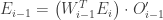
Backpropagation in vector notation
Now write 


Then 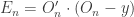

Write 

Then we have 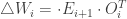


And for the biases write 


Then 
Python Implementation
We will create a class NeuralNetwork and perform our calculations using matrices in numpy.
import numpy as np

class NeuralNetwork(object):
    def __init__(self, X, y, parameters):
        #Input data
        self.X=X
        #Output data
        self.y=y
        #Expect parameters to be a tuple of the form:
        #    ((n_input,0,0), (n_hidden_layer_1, f_1, f_1'), ...,
        #     (n_hidden_layer_k, f_k, f_k'), (n_output, f_o, f_o'))
        self.n_layers = len(parameters)
        #Counts number of neurons without bias neurons in each layer.
        self.sizes = [layer[0] for layer in parameters]
        #Activation functions for each layer.
        self.fs =[layer[1] for layer in parameters]
        #Derivatives of activation functions for each layer.
        self.fprimes = [layer[2] for layer in parameters]
        self.build_network()

    def build_network(self):
        #List of weight matrices taking the output of one layer to the input of the next.
        self.weights=[]
        #Bias vector for each layer.
        self.biases=[]
        #Input vector for each layer.
        self.inputs=[]
        #Output vector for each layer.
        self.outputs=[]
        #Vector of errors at each layer.
        self.errors=[]
        #We initialise the weights randomly, and fill the other vectors with 1s.
        for layer in range(self.n_layers-1):
            n = self.sizes[layer]
            m = self.sizes[layer+1]
            self.weights.append(np.random.normal(0,1, (m,n)))
            self.biases.append(np.random.normal(0,1,(m,1)))
            self.inputs.append(np.zeros((n,1)))
            self.outputs.append(np.zeros((n,1)))
            self.errors.append(np.zeros((n,1)))
        #There are only n-1 weight matrices, so we do the last case separately.
        n = self.sizes[-1]
        self.inputs.append(np.zeros((n,1)))
        self.outputs.append(np.zeros((n,1)))
        self.errors.append(np.zeros((n,1)))

    def feedforward(self, x):
        #Propagates the input from the input layer to the output layer.
        k=len(x)
        x.shape=(k,1)
        self.inputs[0]=x
        self.outputs[0]=x
        for i in range(1,self.n_layers):
            self.inputs[i]=self.weights[i-1].dot(self.outputs[i-1])+self.biases[i-1]
            self.outputs[i]=self.fs[i](self.inputs[i])
        return self.outputs[-1]

    def update_weights(self,x,y):
        #Update the weight matrices for each layer based on a single input x and target y.
        output = self.feedforward(x)
        self.errors[-1]=self.fprimes[-1](self.outputs[-1])*(output-y)

        n=self.n_layers-2
        for i in xrange(n,0,-1):
            self.errors[i] = self.fprimes[i](self.inputs[i])*self.weights[i].T.dot(self.errors[i+1])
            self.weights[i] = self.weights[i]-self.learning_rate*np.outer(self.errors[i+1],self.outputs[i])
            self.biases[i] = self.biases[i] - self.learning_rate*self.errors[i+1]
        self.weights[0] = self.weights[0]-self.learning_rate*np.outer(self.errors[1],self.outputs[0])
        self.biases[0] = self.biases[0] - self.learning_rate*self.errors[1]
    def train(self,n_iter, learning_rate=1):
        #Updates the weights after comparing each input in X with y
        #repeats this process n_iter times.
        self.learning_rate=learning_rate
        n=self.X.shape[0]
        for repeat in range(n_iter):
            #We shuffle the order in which we go through the inputs on each iter.
            index=list(range(n))
            np.random.shuffle(index)
            for row in index:
                x=self.X[row]
                y=self.y[row]
                self.update_weights(x,y)

    def predict_x(self, x):
        return self.feedforward(x)

    def predict(self, X):
        n = len(X)
        m = self.sizes[-1]
        ret = np.ones((n,m))
        for i in range(len(X)):
            ret[i,:] = self.feedforward(X[i])
        return ret
And we’re done! Now to test it we generate some synthetic data and supply the network with some activation functions.
def logistic(x):
    return 1.0/(1+np.exp(-x))

def logistic_prime(x):
    ex=np.exp(-x)
    return ex/(1+ex)**2

def identity(x):
    return x

def identity_prime(x):
    return 1
First we will try to get it to approximate a sine curve.
#expit is a fast way to compute logistic using precomputed exp.
from scipy.special import expit
def test_regression(plots=False):
    #First create the data.
    n=200
    X=np.linspace(0,3*np.pi,num=n)
    X.shape=(n,1)
    y=np.sin(X)
    #We make a neural net with 2 hidden layers, 20 neurons in each, using logistic activation
    #functions.
    param=((1,0,0),(20, expit, logistic_prime),(20, expit, logistic_prime),(1,identity, identity_prime))
    #Set learning rate.
    rates=[0.05]
    predictions=[]
    for rate in rates:
        N=NeuralNetwork(X,y,param)
        N.train(4000, learning_rate=rate)
        predictions.append([rate,N.predict(X)])
    import matplotlib.pyplot as plt
    fig, ax=plt.subplots(1,1)
    if plots:
        ax.plot(X,y, label='Sine', linewidth=2, color='black')
        for data in predictions:
            ax.plot(X,data[1],label="Learning Rate: "+str(data[0]))
        ax.legend()
test_regression(True)
When I ran this it produced the following:

Next we will try a classification problem with a nonlinear decision boundary, how about being above and below the sine curve?
def test_classification(plots=False):
    #Number samples
    n=700

    n_iter=1500
    learning_rate=0.05

    #Samples for true decision boundary plot
    L=np.linspace(0,3*np.pi,num=n)
    l = np.sin(L)

    #Data inputs, training
    X = np.random.uniform(0, 3*np.pi, size=(n,2))
    X[:,1] *= 1/np.pi
    X[:,1]-= 1

    #Data inputs, testing
    T = np.random.uniform(0, 3*np.pi, size=(n,2))
    T[:,1] *= 1/np.pi
    T[:,1] -= 1

    #Data outputs
    y = np.sin(X[:,0]) <= X[:,1]

    #Fitting
    param=((2,0,0),(30, expit, logistic_prime),(30, expit, logistic_prime),(1,expit, logistic_prime))
    N=NeuralNetwork(X,y, param)
    #Training
    N.train(n_iter, learning_rate)
    predictions_training=N.predict(X)
    predictions_training= predictions_training <0.5
    predictions_training= predictions_training[:,0]
    #Testing
    predictions_testing=N.predict(T)
    predictions_testing= predictions_testing <0.5
    predictions_testing= predictions_testing[:,0]

    #Plotting
    import matplotlib.pyplot as plt
    fig, ax=plt.subplots(2,1)

    #Training plot
    #We plot the predictions of the neural net blue for class 0, red for 1.
    ax[0].scatter(X[predictions_training,0], X[predictions_training,1], color='blue')
    not_index = np.logical_not(predictions_training)
    ax[0].scatter(X[not_index,0], X[not_index,1], color='red')
    ax[0].set_xlim(0, 3*np.pi)
    ax[0].set_ylim(-1,1)
    #True decision boundary
    ax[0].plot(L,l, color='black')
    #Shade the areas according to how to they should be classified.
    ax[0].fill_between(L, l,y2=-1, alpha=0.5)
    ax[0].fill_between(L, l, y2=1, alpha=0.5, color='red')

    #Testing plot
    ax[1].scatter(T[predictions_testing,0], T[predictions_testing,1], color='blue')
    not_index = np.logical_not(predictions_testing)
    ax[1].scatter(T[not_index,0], T[not_index,1], color='red')
    ax[1].set_xlim(0, 3*np.pi)
    ax[1].set_ylim(-1,1)
    ax[1].plot(L,l, color='black')
    ax[1].fill_between(L, l,y2=-1, alpha=0.5)
    ax[1].fill_between(L, l, y2=1, alpha=0.5, color='red')

test_classification()
When I ran this it looked like this.

The top plot shows the performance on the training data, and the bottom the performance of on the testing data. The points are colored according to the net’s predictions, whereas the areas are shaded according to the true classifications.
As you can see neural networks are capable of giving very good models, but the number of iterations and hidden nodes may be large. Less iterations are possible using good configurations of the network i terms of sizes and numbers of hidden layers, and choosing the learning rate well, but it is difficult to know how to choose these well.
It ended up being quicker to choose a larger number of hidden nodes, a large number of iterations, and a small learning rate, than to experiment finding a good choice. In the future I may write about how to use momentum to speed up training.
The code for this post is available here, please comment if anything is unclear or incorrect!

Reblogged this on healthcare software solutions lava kafle kathmandu nepal lava prasad kafle lava kafle on google+ <a href="https://plus.google.com/102726194262702292606" rel="publisher">Google+</a>.
[…] with theano, and thanks to gpu computation, much faster also! I recommend having a look at my python implementation of backpropagation just so you can see the effort saved. This implementation benefited greatly from this […]