What’s an abstract simplicial complex?

So what is an abstract simplicial complex? It is a collection of finite sets that are closed under taking subsets.  So if is an abstract simplicial complex (asc), and , then every subset of is also in .

These are meant to be combinatorial models of geometric simplicial complexes, which are topological spaces given by collections of simplices, like a point, a line segment, a triangle or a tetrahedron. An n-simplex is the convex hull of affinely independent points in .

These are important in topology and geometry because they are very easy to understand and compute with, but can be pieced together in clever ways to approximate more complicated objects.

Some terminology

Let be an abs.

Definition: the vertices of , written , are the set of all points in at least one element of . Writing this formally: .

Definition: An element of is called a simplex.

Definition: If is a simplex, and is a subset of , then we say that is a face of or that is a coface of and denote this by .

Definition: If then the dimension of is .

Definition: If and the only coface of is itself, then we call a maximal simplex.

Notice that an abs is completely determined by its set of maximal simplices.

Representation in Python

We want a convenient way to represent and generate these objects. Firstly we want to create one from a list of maximal simplices given as lists of integers. Secondly we want to map the (co)face relations, and enable us to easily iterate over simplices of a given dimension.

So stage one will be unwrapping the maximal simplices into simplices, placing them in a tree. Stage two will be filling in the face relations, representing the abs as a Hasse diagram, where each node represents a simplex.

Stage 1

In our data structure a node represents a simplex. So we create a new node class for the job.

import tigraphs2 as tig
class Simplex(tig.BasicNode, object):
    def __init__(self, vertices, **kwargs):
        super(Simplex, self).__init__(**kwargs)

        self.vertices = vertices
        self.faces=[]
        self.cofaces=[]
        self.dimension = len(self.vertices)-1
        #These are used for initializing the complex:
        self._cfaces =[]
        self._children={}
        self.__parent = None

Now we want to create a class for a complex, which will inherit from the tree class since the initial structure will be a tree.

class SimplicialComplex(tig.return_tree_class(), object):
    def __init__(self, maximal_simplices, Vertex=Simplex, **kwargs):
        super(SimplicialComplex, self).__init__(Vertex=Vertex, **kwargs)
        self.maximal_simplices = maximal_simplices
        self.dimension = max(map(len,self.maximal_simplices))-1
        self.n_simplex_dict={} #Keeps track of simplexes by dimension.
        for i in range(-1,self.dimension+1):
            self.n_simplex_dict[i]=[]
        #Create the empty set 'root' of the structure.
        self.create_simplex([])
        self.set_root(self.vertices[0])
        self.vertices[0].label=str([])
        #Initialize complex from maximal simplices
        for ms in self.maximal_simplices:
            self.add_maximal_simplex(ms)

Now we actually need to write the methods, starting with the create_simplex method:

    def create_simplex(self, vertices):
        self.create_vertex(vertices)
        vertex = self.vertices[-1]
        self.n_simplex_dict[vertex.dimension].append(self.vertices[-1])
        #It is convienient for the simplex to know its index for later on
        #when we create 'vectors' of simplices.
        index = len(self.n_simplex_dict[vertex.dimension])-1
        vertex.index=index
        vertex.label=str(vertices)

The way we will form the initial tree is by building up from the empty set, so we need a way of building up sets.

    def create_child(self, simplex, vertex):
        #This method creates a new simplex which is an immediate coface to the argument
        #simplex. It does so by appending the new vertex to the old simplex's vertices.

        #_cfaces keeps track of which of the simplex's cofaces have already been added.

        if vertex in simplex._cfaces:
            return
        simplex._cfaces.append(vertex)
        child_vertices=[v for v in simplex.vertices]
        child_vertices.append(vertex)
        self.create_simplex(child_vertices)
        child=self.vertices[-1]
        child._parent=simplex
        simplex._children[vertex]=child
        self.leaves.add(child)
        self.create_edge(ends=[simplex, child])
        simplex.cofaces.append(child)
        child.faces.append(simplex)

We are now ready to write the add_maximal_simplex method. It is a recursive procedure, starting with the list representing the maximal simplex, say [0,1,2], we add create cofaces to the root [] with vertices [0], [1] and [2]. To each of these new simplices, we pass on a list of vertices still to be added. To [0] we pass [1,2], to [1] we pass [2], and to [2] we pass [].

In general at each stage we use each vertex remaining in turn to create a child, and pass to that child the vertices yet to be used, that is the vertices remaining greater in value.

    def add_maximal_simplex(self,vertices, simplex=None, first=True):
        #We start at the root.
        if first:
            simplex = self.get_root()

        if len(vertices)>=1: #Condition to terminate recursion.
            for index in range(len(vertices)):
                vertex = vertices[index]
                self.create_child(simplex, vertex)
                self.add_maximal_simplex(simplex=simplex._children[vertex],
                                     vertices=vertices[index+1:],
                                        first=False)

That’s stage 1 complete. Let’s improve the default plot method for the graph class and see if the code is working.

    def plot(self,margin=60):
        A = self.get_adjacency_matrix_as_list()
        g = ig.Graph.Adjacency(A, mode='undirected')
        for vertex in self.vertices:
            if vertex.label !=None:
                #print vertex.label
                index=self.vertices.index(vertex)
                g.vs[index]['label']=vertex.label
        #The layout is designed for trees, so we tell it to set the empty set as the root.
        layout = g.layout("rt", root=0)
        visual_style = {}
        visual_style["vertex_size"] = 20
        visual_style["vertex_label_angle"]=3
        visual_style["vertex_label_dist"] =1
        #We want the root at the bottom of the plot.
        layout.rotate(180)
        ig.plot(g, layout=layout, margin=margin, **visual_style)

Great! Let’s try it out on the tetrahedron. This defined by the maximal simplex [0,1,2,3].

def test(n):
    maximal_simplices = [list(range(n))]
    Sn = SimplicialComplex(maximal_simplices)
    Sn.plot()
test(4)

Producing:

Looking good! Notice that the levels of the tree correspond to simplices of similar dimension and that each simplex’s vertices are in numeric order.

Also notice that many of the (co)face relations are missing, so now we fill them in.

Stage 2
First we add a useful method for accessing a simplex by its list of vertices. This is why we have arranged it so that the vertices are always given in ascending order, so we know exactly what each simplex’s address is.

    def get_simplex(self, address, first=True,simplex=None):
        #We recurse up from the root to the desired simplex.
        if first:
            simplex = self.get_root()
        if len(address)==0:
            return simplex
        if address[0] not in simplex._cfaces:
            return None
        return self.get_simplex(address=address[1:],first=False,
                                simplex=simplex._children[address[0]])

Now we need to add in missing faces and cofaces. To do this we add a method to find a given simplex’s immediate faces, its boundary.

    def _boundary(self,simplex):
        vertices = simplex.vertices
        n = len(vertices)
        boundary=[]
        #Each boundary simplex is found by discarding a single vertex.
        for index in range(n):
            boundary.append(vertices[:index]+vertices[index+1:])
        return boundary

Next we add a simple method for creating a (co)face relation.

    def add_face_coface(self, face, coface):
        #Remember that since the tree was constructed from the empty set up,
        #cofaces are the children in the graph.

        if coface._parent != face:
            self.create_edge([face, coface])
            face.cofaces.append(coface)
            coface.faces.append(face)

Now we simply combine these method to add all of the relations. Recall that in a Hasse diagram, we demonstrate inclusions through transitivity where possible.

    def update_adjacency_simplex(self, simplex):
        boundary_faces = self._boundary(simplex)
        boundary_faces = map(self.get_simplex, boundary_faces)
        for face in boundary_faces:
            self.add_face_coface(face,simplex)

    def update_adjacency(self):
        for i in range(self.dimension+1):
            for simplex in self.n_simplex_dict[i]:
                self.update_adjacency_simplex(simplex)

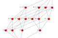
And we’re done! Phew! Now let’s see what it looks like.

def test(n):
    maximal_simplices = [list(range(n))]
    Sn = SimplicialComplex(maximal_simplices)
    Sn.plot()
    Sn.update_adjacency()
    Sn.plot()
test(4)

Producing:

Lovely. You can download the code here, remember you will need igraph for plotting, and my tigraph module from here. Next time we will look at computing the homology of an abs.