Logistic Regression

Welcome back. Last time we showed how to use linear regression to predict a numeric response. Today we are going to talk about what to do if you have a categorical response, like the Titanic data. We will only talk about binary responses, but this method can be extended to cover possible outcomes, and perhaps I will cover that in the future.

Math

We can encode our outcomes as 1 or 0, and we could just run linear regression on this treated as numeric, the problem is that we could get any real  number as a prediction, but we could round this to the nearest 1 or 0. And this sometimes works. But what we might like is for the prediction to always lie in and interpret this as the probability of outcome 1.

To do this we will need to do something nonlinear.  As before let our data be , and now let our binary outcomes be the vector .  Let . Then what we can try is to choose a so that is a good fit for (note I am abusing notation and having act on the vector row-wise).

But what to choose for ? One candidate is called the logistic function, defined , this looks like

(image courtesy of Wikipedia).

Notice how large positive values asymptote to 1, whilst large negative values asymptote to 0. So if these are interpreted as probabilities, the larger the input from the linear combination for some data point , the more certain, one way or the other, our model predicts it is 1 or 0. The decision boundary or cutoff is at zero where the intercept is 0.5. Hence our decision boundary is given by the hyperplane satisfying .

Note that if then this can be rearranged to give , where the left-hand side is called the log-odds in statistics, where ‘odds’ is in the sense of betting odds.

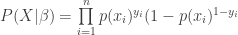
Now previously we just tried to minimise the Euclidean norm of the error, hence the name ‘least-squares regression’. In our case we have predicted probabilities versus binary outcomes, so it is not completely obvious what notion of error to use. We could again use the Euclidean norm, but since we have probabilities, why not choose so that the data we have observed is says maximally probable? This is called maximum likelihood estimation.  If we assume that the observations are independent of one another, then we get

,

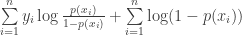
and since products are annoying we look at the log-likelihood

which we can rewrite as

,

plugging in for the log-odds on the left, and on the right gives

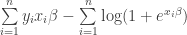
which simplifies finally to

,

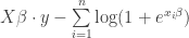
that you might notice is a concave function, and so there are only global maxima, if any.

Now to maximise the log-likelihood we can try differentiate and set to zero, observing that

,

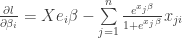
or letting act on a matrix we can write the gradient as

but this will not have a closed form! So we must resort to numerical methods. Since that is not the focus of this post, we will not implement this ourselves, but if you want to do it yourself, you could look at Newton’s method or gradient descent since these are very straightforward to code. I will use something called the truncated newton method, that is found in the scipy library.

Python Implementation

First let’s make up some data to test with. We proceed in a similar fashion to linear regression, but this time instead of trying to predict the y-coordinate from the x, we take both coordinates as our input, and try to predict if the data point is in outcome 1 or 0. Outcome 1 corresponds to points generated by adding a Gaussian noise term to a linear function, and outcome 0 corresponds to points generated by subtracting a Gaussian noise term from the same linear function.

import numpy as np
from scipy import linalg
from scipy import optimize
import random as rd
import matplotlib.pyplot as plt
def test_set(a,b, no_samples, intercept, slope, variance, offset):
    #First we grab some random x-values in the range [a,b].
    X1 = [rd.uniform(a,b) for i in range(no_samples)]
    #Sorting them seems to make the plots work better later on.
    X1.sort()
    #Now we define our linear function that will underly our synthetic dataset: the true decision   boundary.
    def g(x):
        return intercept + slope*x
    #We create two classes of points R,B. R points are given by g(x) plus a Gaussian noise term with positive mean,
    #B points are given by g(x) minus a Gaussian norm term with positive mean.
    R_turn=True
    X2=[] #This will hold the y-coordinates of our data.
    Y=[]  #This will hold the classification of our data.
    for x in X1:
        x2=g(x)
        if R_turn:
            x2 += rd.gauss(offset, variance)
            Y.append(1)
        else:
            x2 -= rd.gauss(offset, variance)
            Y.append(0)
        R_turn=not R_turn
        X2.append(x2)
    #Now we combine the input data into a single matrix.
    X1 = np.array([X1]).T
    X2 = np.array([X2]).T
    X = np.hstack((X1, X2))
    #Now we return the input, output, and true decision boundary.
    return [ X,np.array(Y).T, map(g, X1)]

Fairly straightforward stuff I hope! If not then it should make sense when we plot it.

X,Y,g = test_set(a=0, b=5, no_samples=200, intercept=10, slope=1, variance=2, offset=1)
fig, ax = plt.subplots()
R =  X[::2] #Even terms
B =  X[1::2] #Odd terms

ax.scatter(R[:,0],R[:,1],marker='o', facecolor='red', label="Outcome 1")
ax.scatter(B[:,0],B[:,1],marker='o', facecolor='blue', label="Outcome 0")
ax.plot(X[:,0], g, color='green', label="True Decision Boundary")
ax.legend(loc="upper left", prop={'size':8})
plt.show()

This looks like

so hopefully our decision boundary generated by logistic regression will be close to the true one in green. Note that there could be a better boundary for the random data set shown, but the green line is the one that will generalise best to new data points from the same distribution.

Now that we have some idea what we are doing, we need to code up the functions we want to numerically optimise.

First we make the sigmoid function, which I have previously called , notice that I have coded it in a slightly strange way so as to avoid computing huge numbers ( this idea I got from here).

def sigmoid(x):
    if x>0:
        r = 1/(1. + np.exp(-x))
        return r
    else:
        r = np.exp(x)/(1+np.exp(x))
        return r
vsigmoid= np.vectorize(sigmoid)

The last line there is something I just discovered, vectorisation of functions in numpy! Remember when I abused notation before by having by function act on matrices row wise, or vectors elementwise? Well numpy gives you an extremely convienent way to implement that abuse. Super cool.

Next we write in the log-likelihood or ‘cost’, since the algorithm I want to use is for minimising, we will take the negative of (1):

def cost(beta,X,Y):
    #Function to be minimised.
    p = vsigmoid(X.dot(beta))
    ret = -Y*np.log(p) -(1-Y)*np.log(1-p)
    return ret.sum()

Similarly we will take the negative of the gradient as in (2):

def grad(beta,X,Y):
    p = vsigmoid(X.dot(beta))
    r =  p-Y
    return r.T.dot(X)

And that is really all of the hardwork we have to do! All that remains to write a wrapper to some numerical optimisation function from the scipy library. Note that it took some experimentation to realise that this function wants its numpy vectors ‘flattened’, that is with shape = (n,), not (n,1)! My thanks to this postfor helping me figure this out!

def logistic_regression(X, Y):
    #Initialise beta to something random, that way if it fails to converge
    #you can rerun and get a better result.
    beta = 0.1* numpy.random.randn(X.shape[1])
    #The args argument tells fmin_tnc what to pass to cost and fprime in addition to beta.
    return optimize.fmin_tnc(cost, beta, fprime=grad, args=(X,Y))

And we are done! Now let’s see how it fares on our data set. Remember that once we have our 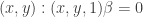, the decision boundary is given by the points .

X1 = np.hstack((X, np.ones((X.shape[0], 1), dtype=X.dtype)))
beta=logistic_regression(X1, Y)
beta=beta[0] #The rest of the tupe has convergence information.
def decision_boundary(x):
    return -x*beta[0]/beta[1] - beta[2]/beta[1]

where the decision boundary function comes from solving for .

Now to display the information I will create two plots side by side. The first will show our decision boundary, the true decision boundary and all the data with its true classification shown by colour.
The other one will show the fitted decision boundary along with the data points, but this time the colors will indicate the predicted probabilities of their classifications: brighter reds and blues correspond to confident predictions of outcomes 1 and 0 respectively, and the colours get lighter as we approach the decision boundary.

fig, (ax1,ax2) = plt.subplots(1,2, sharey=True, sharex=True)
D=[decision_boundary(x) for x in X1[:,0]] #Predicted decision boundary

#Recall we defined R, B earlier as the odd and even data points which correspond to the 2 outcomes.
ax1.scatter(R[:,0],R[:,1],marker='o',facecolor='red',s=50, label="Outcome 1")
ax1.scatter(B[:,0],B[:,1],marker='o', facecolor='blue',s=50, label="Outcome 0")
ax1.plot(X1[:,0], g, '-', color='yellow', linewidth=3, label="True decision boundary")
ax1.plot(X1[:,0], D,linewidth=3, color='black',label="Fitted decision boundary")

#Predicted probability of being red given by model
P = X1.dot(beta)
P = vsigmoid(P)
colors = plt.cm.coolwarm(P)
ax2.scatter(X1[:,0],X1[:,1],marker='o',s=50,facecolors=colors, label="Predicted probability" )

#ax2.plot(X1[:,0], g, '-', color='yellow', linewidth=3, label="True decision boundary")
ax2.plot(X1[:,0], D,linewidth=3, color='black',label="Fitted decision boundary")
legend = ax1.legend(loc='lower right', shadow=True, prop={'size':10})
legend = ax2.legend(loc='lower right', shadow=True, prop={'size':12})
fig.set_size_inches(15,7)

and this will look like:

I hope you have learned something, the ipython notebook for this post is here, and the python code is here.